物理信息网络 PINN:利用神经网络求解偏微分方程
偏微分方程(PDE)是描述物理世界的基本语言——热传导、流体动力学、量子力学,无一不是 PDE 的天下。但求解 PDE 常常需要复杂的数值方法(有限元、有限差分……),对几何形状不规则的区域更是头疼。Physics-Informed Neural Networks(PINN) 给出了一个全新的思路:用神经网络作为 PDE 的解函数,用自动微分作为物理约束的执行器。
1. 什么是 PINN?
PINN 的核心思想:不把神经网络当作”万能拟合器”,而是当作 PDE 解函数的表示。
传统方法:给定边界条件和初始条件,用数值差分近似 PDE 的导数。
PINN:用一个神经网络 u_θ(x,t) 来近似 PDE 的解 u(x,t),其中 θ 是网络权重。通过自动微分(Autodiff)精确计算 PDE 的残差,将其加入损失函数。
2. PINN 架构一览
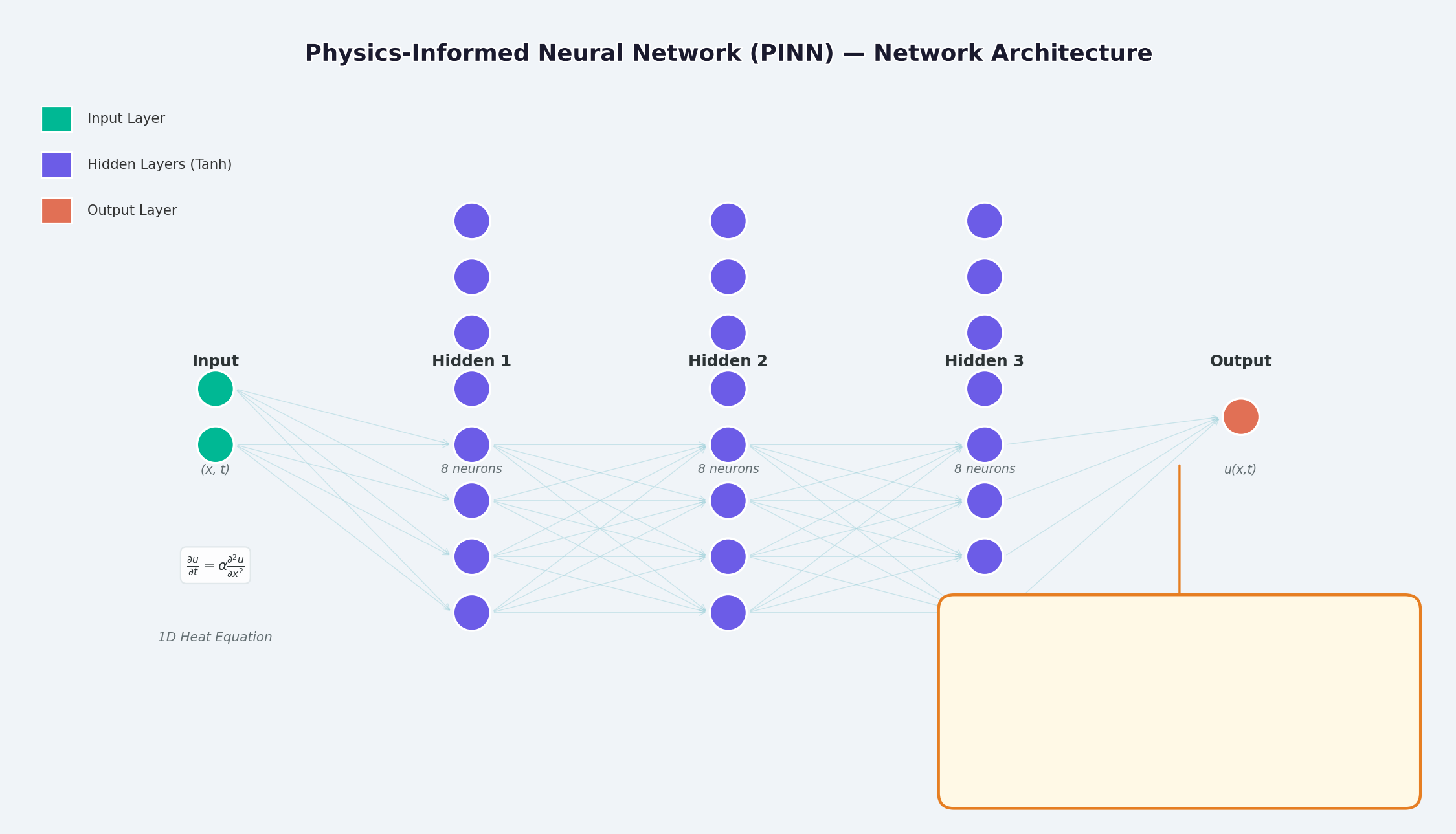
如上图所示,PINN 的结构为:
- 输入层:时空坐标
(x, t) - 隐藏层:全连接层 + 激活函数(Tanh / Sigmoid)
- 输出层:PDE 的解
u(x,t)
关键区别在于损失函数的设计——除了数据拟合损失外,还加入了物理约束损失。
3. 数学原理
3.1 问题设定
以一维热传导方程为例:
边界条件:
初始条件:
3.2 损失函数
PINN 的总损失由三部分组成:
其中 PDE 残差为:
这里的
f(x,t)被称为残差网络(physics network),它完全由自动微分构造,不需要任何有限差分近似。
4. PyTorch 实现
4.1 环境准备
conda activate carlaTest
# carlaTest 已包含: PyTorch 2.4.1 + CUDA + Matplotlib
4.2 完整代码
import torch
import numpy as np
import matplotlib.pyplot as plt
from matplotlib.animation import FuncAnimation
from IPython.display import HTML, Image

device = torch.device("cuda" if torch.cuda.is_available() else "cpu")
print(f"Running on: {device}")

# ============================================================
# 1. 定义 PINN 模型
# ============================================================
class PINN(torch.nn.Module):
    """Physics-Informed Neural Network"""
    def __init__(self, layers=[2, 32, 32, 32, 1]):
        super().__init__()
        # Xavier 初始化
        self.fc = torch.nn.ModuleList([
            torch.nn.Linear(layers[i], layers[i+1])
            for i in range(len(layers)-1)
        ])
        self.apply(self._init_weights)

    def _init_weights(self, m):
        if isinstance(m, torch.nn.Linear):
            torch.nn.init.xavier_normal_(m.weight)
            torch.nn.init.zeros_(m.bias)

    def forward(self, x):
        for i, fc in enumerate(self.fc[:-1]):
            x = torch.tanh(fc(x))      # Tanh 激活
        return self.fc[-1](x)            # 线性输出

# ============================================================
# 2. 精确解(用于对比)
# ============================================================
alpha = 0.01  # 热扩散系数

def exact_solution(x, t):
    """热传导方程解析解: u(x,t) = exp(-π²αt)·sin(πx)"""
    return np.exp(-np.pi**2 * alpha * t) * np.sin(np.pi * x)

# ============================================================
# 3. 训练函数
# ============================================================
def train_pinn(n_iterations=2000, lr=1e-3):
    model = PINN().to(device)
    optimizer = torch.optim.Adam(model.parameters(), lr=lr)

    history = {"total": [], "pde": [], "ic": [], "bc": []}

    for it in range(n_iterations):
        # --- PDE 残差点(内部采样)---
        x_pde = (torch.rand(256, 1, device=device) * 2 - 1).requires_grad_(True)
        t_pde = (torch.rand(256, 1, device=device)).requires_grad_(True)

        # --- 初始条件点(t=0)---
        x_ic = (torch.rand(64, 1, device=device) * 2 - 1)
        t_ic = torch.zeros(64, 1, device=device)

        # --- 边界条件点(x=±1)---
        sign = torch.randint(0, 2, (64, 1), device=device).float() * 2 - 1
        x_bc = sign  # x = +1 或 x = -1
        t_bc = torch.rand(64, 1, device=device)

        # --- 计算 PDE 残差 ---
        xt_pde = torch.cat([x_pde, t_pde], dim=1)
        u = model(xt_pde)

        # 自动微分:计算 u_t 和 u_xx
        u_t = torch.autograd.grad(u, t_pde,
                                 grad_outputs=torch.ones_like(u),
                                 create_graph=True)[0]
        u_x = torch.autograd.grad(u, x_pde,
                                 grad_outputs=torch.ones_like(u),
                                 create_graph=True)[0]
        u_xx = torch.autograd.grad(u_x, x_pde,
                                   grad_outputs=torch.ones_like(u_x),
                                   create_graph=True)[0]

        f = u_t - alpha * u_xx  # = 0 (当网络收敛到正确解时)

        # --- 计算各部分损失 ---
        loss_pde = torch.mean(f**2)

        # 初始条件损失
        u_ic = model(torch.cat([x_ic, t_ic], dim=1))
        u_ic_exact = torch.sin(np.pi * x_ic)
        loss_ic = torch.mean((u_ic - u_ic_exact)**2)

        # 边界条件损失
        u_bc = model(torch.cat([x_bc, t_bc], dim=1))
        loss_bc = torch.mean(u_bc**2)

        # 总损失
        loss = loss_pde + loss_ic + loss_bc

        # 反向传播
        optimizer.zero_grad()
        loss.backward()
        optimizer.step()

        # 记录历史
        if it % 50 == 0:
            history["total"].append(loss.item())
            history["pde"].append(loss_pde.item())
            history["ic"].append(loss_ic.item())
            history["bc"].append(loss_bc.item())

    return model, history

# ============================================================
# 4. 训练
# ============================================================
print("开始训练 PINN...")
model, history = train_pinn(n_iterations=2000)
print(f"最终损失: {history['total'][-1]:.6f}")
4.3 可视化:训练过程
# === 训练损失分解动画 ===
fig, axes = plt.subplots(1, 2, figsize=(14, 5))

def animate(frame):
    step = max(1, len(history["total"]) // 50)
    idx = min(frame * step, len(history["total"])-1)

    axes[0].cla()
    axes[1].cla()

    iters = np.arange(len(history["total"])) * 50
    pde_ls = history["pde"]
    ic_ls  = history["ic"]
    bc_ls  = history["bc"]

    # 左图:堆叠面积图
    axes[0].fill_between(iters[:idx+1], pde_ls[:idx+1], alpha=0.4, color="#FF6B6B", label="PDE 损失")
    axes[0].fill_between(iters[:idx+1], np.array(pde_ls[:idx+1])+np.array(ic_ls[:idx+1]),
                              alpha=0.4, color="#4ECDC4", label="初始条件损失")
    axes[0].fill_between(iters[:idx+1],
                         np.array(pde_ls[:idx+1])+np.array(ic_ls[:idx+1])+np.array(bc_ls[:idx+1]),
                              alpha=0.4, color="#45B7D1", label="边界条件损失")
    axes[0].set_yscale("log")
    axes[0].set_xlabel("迭代次数")
    axes[0].set_ylabel("损失值 (对数坐标)")
    axes[0].legend(loc="upper right")
    axes[0].grid(True, alpha=0.3)
    axes[0].set_title("损失分量演化(堆叠面积图)")

    # 右图:分线对比
    axes[1].semilogy(iters[:idx+1], pde_ls[:idx+1], "r-",  lw=2, label="PDE")
    axes[1].semilogy(iters[:idx+1], ic_ls[:idx+1],  "g--", lw=2, label="初始条件")
    axes[1].semilogy(iters[:idx+1], bc_ls[:idx+1],  "b:",  lw=2, label="边界条件")
    axes[1].scatter([iters[idx]], [history["total"][idx]], color="purple", s=100, zorder=5)
    axes[1].set_xlabel("迭代次数")
    axes[1].set_ylabel("损失值 (对数坐标)")
    axes[1].legend(loc="upper right")
    axes[1].grid(True, alpha=0.3)
    axes[1].set_title("各损失分量对比")

ani = FuncAnimation(fig, animate, frames=50, interval=150)
ani.save("pinn_loss_components.gif", writer="pillow", fps=6, dpi=100)
5. 可视化结果
5.1 解的收敛过程
上图展示了 PINN 在训练过程中逐步逼近精确解的过程:
- 左图:t=0.5 时刻的解曲线,红色虚线为 PINN 预测,蓝色实线为精确解
- 中图:训练损失(对数坐标),可以看到三种损失协同下降
- 右图:PINN 预测的完整 (x,t) 解场
5.2 损失函数分解
从损失分解动画可以看出:
- PDE 损失(红色)下降最快,说明网络快速学到了物理规律
- 边界条件损失(蓝色) 通常最小,因为边界条件约束最简单
- 三种损失最终趋于稳定,表明网络已收敛
6. PINN 的优势
| 特性 | 传统数值方法(FEM/FDM) | PINN |
|---|---|---|
| 网格生成 | 需要精细网格,高维困难 | 无需网格,随机采样 |
| 导数精度 | 依赖差分近似,有截断误差 | 自动微分,任意精度 |
| 不规则区域 | 网格划分复杂 | 天然支持任意几何 |
| 反问题 | 需要重求解器 | 端到端梯度优化 |
| 高维问题 | 维度灾难 | Scalable |
7. PINN 的局限与挑战
PINN 并非万能药——它有自己独特的局限。
7.1 训练困难
- 模式坍缩(Mode Collapse):当 PDE 有多个解时,PINN 可能只学到其中一个
- 梯度消失:高阶导数(如 u_xxxx)的梯度在深层网络中可能极小
- 超参数敏感:网络深度、学习率、采样策略对结果影响显著
7.2 解的精度
- 神经网络在高频解(如震荡解)上精度较差
- 边界层、奇异性附近需要特殊处理(自适应采样、周期扩展等)
7.3 计算效率
- 相比成熟数值库(如 FEniCS、COMSOL),PINN 在简单 PDE 上往往更慢
- GPU 利用率不如专用数值代码高
7.4 改进方向
- Adaptive Sampling:在误差大的区域多采样(如 Residual-based Adaptive Refinement)
- DeepONet: Operator Network,直接学习 PDE 解算子
- Fourier Neural Operator (FNO):频域神经算子,高维问题效果更好
- HP-VPINN:基于变分形式的 PINN,精度更高
8. 完整训练代码(可运行)
"""
PINN 求解一维热传导方程
conda activate carlaTest
python pinn_heat_equation.py
"""
import torch, numpy as np, matplotlib.pyplot as plt

device = torch.device("cuda" if torch.cuda.is_available() else "cpu")
alpha = 0.01

class PINN(torch.nn.Module):
    def __init__(self):
        super().__init__()
        self.net = torch.nn.Sequential(
            torch.nn.Linear(2, 32), torch.nn.Tanh(),
            torch.nn.Linear(32, 32), torch.nn.Tanh(),
            torch.nn.Linear(32, 32), torch.nn.Tanh(),
            torch.nn.Linear(32, 1)
        )
    def forward(self, x):
        return self.net(x)

model = PINN().to(device)
opt = torch.optim.Adam(model.parameters(), lr=1e-3)

for it in range(2000):
    x_pde = (torch.rand(256,1,device=device)*2-1).requires_grad_(True)
    t_pde = (torch.rand(256,1,device=device)).requires_grad_(True)
    x_ic  = (torch.rand(64,1,device=device)*2-1)
    t_ic  = torch.zeros(64,1,device=device)
    x_bc  = (torch.randint(0,2,(64,1),device=device).float()*2-1)
    t_bc  = torch.rand(64,1,device=device)

    xt = torch.cat([x_pde,t_pde],dim=1)
    u = model(xt)
    u_t  = torch.autograd.grad(u,t_pde,torch.ones_like(u),create_graph=True)[0]
    u_x  = torch.autograd.grad(u,x_pde,torch.ones_like(u),create_graph=True)[0]
    u_xx = torch.autograd.grad(u_x,x_pde,torch.ones_like(u_x),create_graph=True)[0]

    loss = (torch.mean((u_t-alpha*u_xx)**2)
             + torch.mean((model(torch.cat([x_ic,t_ic],1))-torch.sin(np.pi*x_ic))**2)
             + torch.mean(model(torch.cat([x_bc,t_bc],1))**2))

    opt.zero_grad(); loss.backward(); opt.step()
    if it%200==0: print(f"Iter {it:5d} | Loss: {loss.item():.6f}")

# 测试
x_test = torch.linspace(-1,1,100,device=device).reshape(-1,1)
t_test = torch.ones(100,1,device=device)*0.5
u_pred = model(torch.cat([x_test,t_test],1)).cpu().detach().numpy()
u_true = np.exp(-np.pi**2*alpha*0.5)*np.sin(np.pi*x_test.cpu().numpy())

plt.figure(figsize=(8,4))
plt.plot(x_test.cpu(),u_true,"b-",lw=2,label="精确解")
plt.plot(x_test.cpu(),u_pred,"r--",lw=2,label="PINN 预测")
plt.legend(); plt.title("t=0.5 时刻的热传导方程解")
plt.savefig("pinn_result.png",dpi=150)
print("结果已保存!")
9. 总结
PINN 将物理先验嵌入神经网络的训练过程,开辟了”物理驱动的深度学习”这一新范式。它的核心创新不是网络结构,而是损失函数的设计——用自动微分精确施加物理约束。
尽管存在训练困难、精度有限等挑战,PINN 在以下场景中展现了独特价值:
- 高维 PDE(传统方法维度灾难)
- 反问题(参数识别、数据同化)
- 不确定性量化(结合贝叶斯方法)
如果你想进一步探索,推荐从 DeepXDE 库开始,它封装了大量 PINN 变体和自适应采样策略。
参考论文:
- Raissi, M., Perdikaris, P., & Karniadakis, G. E. (2019). Physics-informed neural networks: A deep learning framework for solving forward and inverse problems involving nonlinear partial differential equations. Journal of Computational Physics, 378, 686-707.
- Lu, L., et al. (2021). DeepONet: Learning nonlinear operators for identifying differential equations based on the universal approximation theorem of operators. Nature Machine Intelligence, 3(3), 218-229.
- Li, Z., Kovachki, N., Azizzadenesheli, K., Liu, B., Bhattacharya, K., Stuart, A., & Anandkumar, A. (2020). Fourier neural operator for parametric partial differential equations. arXiv preprint arXiv:2010.08895.