物理情報ネットワーク PINN: ニューラル ネットワークを使用して偏微分方程式を解く

原理からコードに至るまでの物理情報に基づいたニューラル ネットワークの詳細な分析により、PyTorch を使用して PINN を実装する方法を段階的に説明し、トレーニング プロセスを視覚化します。

Physical Information Network PINN: ニューラルネットワークを使用して偏微分方程式を解く

偏微分方程式 (PDE) は、熱伝導、流体力学、量子力学などの物理世界を記述するための基本言語であり、それらはすべて PDE によって支配されます。ただし、偏微分方程式を解くには複雑な数値手法 (有限要素、有限差分など) が必要になることが多く、不規則な幾何学的形状を持つ領域ではさらに困難になります。 物理情報に基づいたニューラル ネットワーク (PINN) は、ニューラル ネットワークを PDE の解関数として使用し、 自動微分を物理的制約のアクチュエーターとして使用するというまったく新しいアイデアを提供します。


##1.PINNとは何ですか?

PINN の中心的な考え方: ニューラル ネットワークを「ユニバーサル フィッター」としてではなく、 PDE 解関数の表現 として扱います。

従来の方法: 与えられた境界条件と初期条件を使用して、数値の差を使用して偏微分方程式の導関数を近似します。

PINN: ニューラル ネットワーク u_θ(x,t) を使用して偏微分方程式 u(x,t) の解を近似します。ここで、θ はネットワークの重みです。 PDE の残差は自動微分 (Autodiff) によって正確に計算され、損失関数に追加されます。


2. PINN アーキテクチャの概要
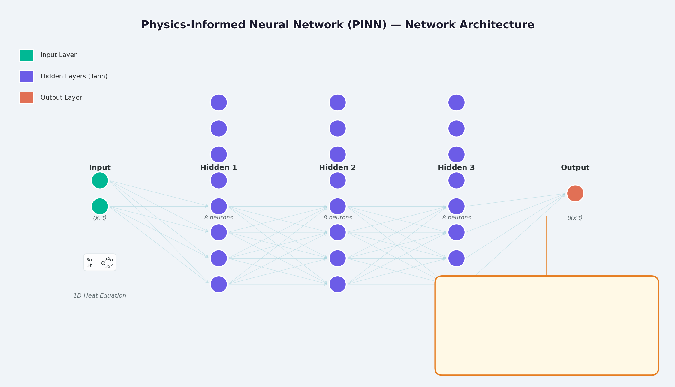
PINN アーキテクチャ

上の図に示すように、PINN の構造は次のとおりです。

主な違いは損失関数の設計にあります。データ フィッティング損失に加えて、物理的制約損失も追加されます。


3. 数学的原理

3.1 問題設定

例として一次元の熱伝導方程式を考えてみましょう。

u(-1, t) = u(1, t) = 0

u(x, 0) = \sin(\pi x)

You can't use 'macro parameter character #' in math mode ### 3.2 損失関数 PINN の合計損失は 3 つの部分で構成されます。

\mathcal{L}{合計} = \underbrace{\mathcal{L}{PDE}}{\text{方程式残差}} + \underbrace{\mathcal{L}{IC}}{\text{初期条件}} + \underbrace{\mathcal{L}{BC}}_{\text{境界条件}}

f(x,t) = \frac{\partial u}{\partial t} - \alpha \frac{\partial^2 u}{\partial x^2} \quad \Rightarrow \quad \mathcal{L}{PDE} = \frac{1}{N}\sum{i=1}^{N} |f(x_i, t_i)|^2

You can't use 'macro parameter character #' in math mode > ここでの「f(x,t)」 は<strong>残差ネットワーク(物理ネットワーク)</strong>と呼ばれるもので、完全に自動微分によって構築され、有限差分近似は必要ありません。 --- ## 4. PyTorch の実装 ### 4.1 環境の準備 ```bash conda activate carlaTest # carlaTest 已包含: PyTorch 2.4.1 + CUDA + Matplotlib ``` ### 4.2 完全なコード ```python import torch import numpy as np import matplotlib.pyplot as plt from matplotlib.animation import FuncAnimation from IPython.display import HTML, Image device = torch.device("cuda" if torch.cuda.is_available() else "cpu") print(f"Running on: {device}") # ============================================================ # 1. 定义 PINN 模型 # ============================================================ class PINN(torch.nn.Module): """Physics-Informed Neural Network""" def __init__(self, layers=[2, 32, 32, 32, 1]): super().__init__() # Xavier 初始化 self.fc = torch.nn.ModuleList([ torch.nn.Linear(layers[i], layers[i+1]) for i in range(len(layers)-1) ]) self.apply(self._init_weights) def _init_weights(self, m): if isinstance(m, torch.nn.Linear): torch.nn.init.xavier_normal_(m.weight) torch.nn.init.zeros_(m.bias) def forward(self, x): for i, fc in enumerate(self.fc[:-1]): x = torch.tanh(fc(x)) # Tanh 激活 return self.fc[-1](x) # 线性输出 # ============================================================ # 2. 精确解(用于对比) # ============================================================ alpha = 0.01 # 热扩散系数 def exact_solution(x, t): """热传导方程解析解: u(x,t) = exp(-π²αt)·sin(πx)""" return np.exp(-np.pi**2 * alpha * t) * np.sin(np.pi * x) # ============================================================ # 3. 训练函数 # ============================================================ def train_pinn(n_iterations=2000, lr=1e-3): model = PINN().to(device) optimizer = torch.optim.Adam(model.parameters(), lr=lr) history = {"total": [], "pde": [], "ic": [], "bc": []} for it in range(n_iterations): # --- PDE 残差点(内部采样)--- x_pde = (torch.rand(256, 1, device=device) * 2 - 1).requires_grad_(True) t_pde = (torch.rand(256, 1, device=device)).requires_grad_(True) # --- 初始条件点(t=0)--- x_ic = (torch.rand(64, 1, device=device) * 2 - 1) t_ic = torch.zeros(64, 1, device=device) # --- 边界条件点(x=±1)--- sign = torch.randint(0, 2, (64, 1), device=device).float() * 2 - 1 x_bc = sign # x = +1 或 x = -1 t_bc = torch.rand(64, 1, device=device) # --- 计算 PDE 残差 --- xt_pde = torch.cat([x_pde, t_pde], dim=1) u = model(xt_pde) # 自动微分:计算 u_t 和 u_xx u_t = torch.autograd.grad(u, t_pde, grad_outputs=torch.ones_like(u), create_graph=True)[0] u_x = torch.autograd.grad(u, x_pde, grad_outputs=torch.ones_like(u), create_graph=True)[0] u_xx = torch.autograd.grad(u_x, x_pde, grad_outputs=torch.ones_like(u_x), create_graph=True)[0] f = u_t - alpha * u_xx # = 0 (当网络收敛到正确解时) # --- 计算各部分损失 --- loss_pde = torch.mean(f**2) # 初始条件损失 u_ic = model(torch.cat([x_ic, t_ic], dim=1)) u_ic_exact = torch.sin(np.pi * x_ic) loss_ic = torch.mean((u_ic - u_ic_exact)**2) # 边界条件损失 u_bc = model(torch.cat([x_bc, t_bc], dim=1)) loss_bc = torch.mean(u_bc**2) # 总损失 loss = loss_pde + loss_ic + loss_bc # 反向传播 optimizer.zero_grad() loss.backward() optimizer.step() # 记录历史 if it % 50 == 0: history["total"].append(loss.item()) history["pde"].append(loss_pde.item()) history["ic"].append(loss_ic.item()) history["bc"].append(loss_bc.item()) return model, history # ============================================================ # 4. 训练 # ============================================================ print("开始训练 PINN...") model, history = train_pinn(n_iterations=2000) print(f"最终损失: {history['total'][-1]:.6f}") ``` ### 4.3 視覚化: トレーニング プロセス ```python # === 训练损失分解动画 === fig, axes = plt.subplots(1, 2, figsize=(14, 5)) def animate(frame): step = max(1, len(history["total"]) // 50) idx = min(frame * step, len(history["total"])-1) axes[0].cla() axes[1].cla() iters = np.arange(len(history["total"])) * 50 pde_ls = history["pde"] ic_ls = history["ic"] bc_ls = history["bc"] # 左图:堆叠面积图 axes[0].fill_between(iters[:idx+1], pde_ls[:idx+1], alpha=0.4, color="#FF6B6B", label="PDE 损失") axes[0].fill_between(iters[:idx+1], np.array(pde_ls[:idx+1])+np.array(ic_ls[:idx+1]), alpha=0.4, color="#4ECDC4", label="初始条件损失") axes[0].fill_between(iters[:idx+1], np.array(pde_ls[:idx+1])+np.array(ic_ls[:idx+1])+np.array(bc_ls[:idx+1]), alpha=0.4, color="#45B7D1", label="边界条件损失") axes[0].set_yscale("log") axes[0].set_xlabel("迭代次数") axes[0].set_ylabel("损失值 (对数坐标)") axes[0].legend(loc="upper right") axes[0].grid(True, alpha=0.3) axes[0].set_title("损失分量演化(堆叠面积图)") # 右图:分线对比 axes[1].semilogy(iters[:idx+1], pde_ls[:idx+1], "r-", lw=2, label="PDE") axes[1].semilogy(iters[:idx+1], ic_ls[:idx+1], "g--", lw=2, label="初始条件") axes[1].semilogy(iters[:idx+1], bc_ls[:idx+1], "b:", lw=2, label="边界条件") axes[1].scatter([iters[idx]], [history["total"][idx]], color="purple", s=100, zorder=5) axes[1].set_xlabel("迭代次数") axes[1].set_ylabel("损失值 (对数坐标)") axes[1].legend(loc="upper right") axes[1].grid(True, alpha=0.3) axes[1].set_title("各损失分量对比") ani = FuncAnimation(fig, animate, frames=50, interval=150) ani.save("pinn_loss_components.gif", writer="pillow", fps=6, dpi=100) ``` --- ## 5. 結果を視覚化する ### 5.1 解の収束プロセス ![PINN 収束アニメーション](/pinn_gifs/pinn_convergence.gif) 上の図は、トレーニング プロセス中に PINN が徐々に正確な解に近づいていくプロセスを示しています。 - <strong>左の図</strong>: 時間 t=0.5 での解曲線、赤い点線は PINN 予測、青い実線は正確な解です。 - <strong>中央の図</strong>: トレーニング損失 (対数スケール)。3 つの損失が協調して減少していることがわかります。 - <strong>右の画像</strong>: PINN によって予測された完全な (x,t) 解フィールド ### 5.2 損失関数の分解![PINN 損失分解アニメーション](/pinn_gifs/pinn_loss_components.gif) 損失分解アニメーションからわかるように、次のようになります。 - <strong>PDE 損失 (赤)</strong> が最も速く低下し、ネットワークが物理法則をすぐに学習したことを示しています - 境界条件制約が最も単純であるため、<strong>境界条件損失 (青)</strong> は通常最小になります。 - 3 つの損失は最終的に安定し、ネットワークが収束したことを示します。 --- ## 6. PINN の利点 |プロパティ |従来の数値手法 (FEM/FDM) |ピン | |------|-------------|------| |グリッドの生成 |細かいグリッドが必要、高次元化は難しい | <strong>グリッドは不要</strong>、ランダムサンプリング | |微分精度 |微分近似に依存しており、切り捨て誤差がある | <strong>自動微分</strong>、任意精度 | |不規則な領域 |複雑なメッシュ |任意のジオメトリの<strong>自然なサポート</strong> | |逆問題 |リソルバーが必要 | <strong>エンドツーエンド</strong>の勾配最適化 | |高次元の問題 |次元の呪い | <strong>スケーラブル</strong> | --- ## 7. PINN の限界と課題 > PINN は万能薬ではありません。PINN には独自の制限があります。 ### 7.1 トレーニングの難しさ - <strong>モード崩壊</strong>: PDE に複数の解がある場合、PINN はそのうちの 1 つだけを学習する可能性があります。 - <strong>勾配消失</strong>: 高次導関数 (u_xxxx など) の勾配は、深いネットワークでは非常に小さい場合があります。 - <strong>ハイパーパラメータ感度</strong>: ネットワークの深さ、学習率、サンプリング戦略は結果に大きな影響を与えます。 ### 7.2 解の精度 - ニューラル ネットワークは<strong>高周波解</strong>(振動解など)では精度が低くなります。 - 境界層と特異点には特別な処理(適応サンプリング、周期拡張など)が必要です。 ### 7.3 計算効率 - PINN は、成熟した数値ライブラリ (FEniCS、COMSOL など) よりも単純な偏微分方程式では<strong>遅い</strong>傾向があります。 - GPU 使用率は専用の数値コードほど高くありません ### 7.4 改善の方向性- <strong>適応サンプリング</strong>: 誤差が大きい領域でのマルチサンプリング (残差ベースの適応リファインメントなど) - <strong>DeepONEt</strong>: オペレーター ネットワーク、PDE ソリューション オペレーターを直接学習します - <strong>フーリエ ニューラル演算子 (FNO)</strong>: 周波数領域のニューラル演算子。高次元の問題に適しています。 - <strong>HP-VPINN</strong>: 変分形式に基づく PINN、より高い精度 --- ## 8. 完全なトレーニング コード (実行準備完了) ```python """ PINN 求解一维热传导方程 conda activate carlaTest python pinn_heat_equation.py """ import torch, numpy as np, matplotlib.pyplot as plt device = torch.device("cuda" if torch.cuda.is_available() else "cpu") alpha = 0.01 class PINN(torch.nn.Module): def __init__(self): super().__init__() self.net = torch.nn.Sequential( torch.nn.Linear(2, 32), torch.nn.Tanh(), torch.nn.Linear(32, 32), torch.nn.Tanh(), torch.nn.Linear(32, 32), torch.nn.Tanh(), torch.nn.Linear(32, 1) ) def forward(self, x): return self.net(x) model = PINN().to(device) opt = torch.optim.Adam(model.parameters(), lr=1e-3) for it in range(2000): x_pde = (torch.rand(256,1,device=device)*2-1).requires_grad_(True) t_pde = (torch.rand(256,1,device=device)).requires_grad_(True) x_ic = (torch.rand(64,1,device=device)*2-1) t_ic = torch.zeros(64,1,device=device) x_bc = (torch.randint(0,2,(64,1),device=device).float()*2-1) t_bc = torch.rand(64,1,device=device) xt = torch.cat([x_pde,t_pde],dim=1) u = model(xt) u_t = torch.autograd.grad(u,t_pde,torch.ones_like(u),create_graph=True)[0] u_x = torch.autograd.grad(u,x_pde,torch.ones_like(u),create_graph=True)[0] u_xx = torch.autograd.grad(u_x,x_pde,torch.ones_like(u_x),create_graph=True)[0] loss = (torch.mean((u_t-alpha*u_xx)**2) + torch.mean((model(torch.cat([x_ic,t_ic],1))-torch.sin(np.pi*x_ic))**2) + torch.mean(model(torch.cat([x_bc,t_bc],1))**2)) opt.zero_grad(); loss.backward(); opt.step() if it%200==0: print(f"Iter {it:5d} | Loss: {loss.item():.6f}") # 测试 x_test = torch.linspace(-1,1,100,device=device).reshape(-1,1) t_test = torch.ones(100,1,device=device)*0.5 u_pred = model(torch.cat([x_test,t_test],1)).cpu().detach().numpy() u_true = np.exp(-np.pi**2*alpha*0.5)*np.sin(np.pi*x_test.cpu().numpy()) plt.figure(figsize=(8,4)) plt.plot(x_test.cpu(),u_true,"b-",lw=2,label="精确解") plt.plot(x_test.cpu(),u_pred,"r--",lw=2,label="PINN 预测") plt.legend(); plt.title("t=0.5 时刻的热传导方程解") plt.savefig("pinn_result.png",dpi=150) print("结果已保存!") ``` --- ## 9. まとめ PINN はニューラル ネットワークのトレーニング プロセスに<strong>物理的な事前分布</strong>を埋め込み、「物理駆動型ディープラーニング」の新しいパラダイムを開きます。その中心となる革新はネットワーク構造ではなく、自動微分による物理的制約を正確に課す損失関数の設計です。 トレーニングの難しさや精度の限界などの課題にもかかわらず、PINN は次のシナリオで独自の価値を実証しました。 - <strong>高次元偏微分方程式</strong> (従来の手法の次元災害) - <strong>逆問題</strong> (パラメータの同定、データの同化) - <strong>不確実性の定量化</strong> (ベイジアン手法との組み合わせ) > さらに詳しく調べたい場合は、[DeepXDE](https://deepxde.readthedocs.io/) ライブラリから始めることをお勧めします。このライブラリには、多数の PINN バリアントと適応サンプリング戦略がカプセル化されています。 ---<strong>参考文献:</strong> 1. Raissi, M.、Perdicaris, P.、Karniadakis, G.E. (2019)。 *物理情報に基づいたニューラル ネットワーク: 非線形偏微分方程式を含む順問題および逆問題を解決するための深層学習フレームワーク。* Journal of Computational Physics、378、686-707。 2. Lu、L.、他。 (2021年)。 *DeepONet: 演算子の普遍近似定理に基づいて微分方程式を特定するための非線形演算子の学習。* Nature Machine Intelligence、3(3)、218-229。 3. Li, Z.、Kovachki, N.、Azizzadenesheli, K.、Liu, B.、Bhattacharya, K.、Stuart, A.、および Anandkumar, A. (2020)。 *パラメトリック偏微分方程式のフーリエ ニューラル演算子。* arXiv プレプリント arXiv:2010.08895。