Physical Information Network PINN: Solving partial differential equations using neural networks In-depth analysis of Physics-Informed Neural Networks, from principles to code, teaches you step by step how to implement PINN using PyTorch, and visualizes the training process
deep learning PDE PINN PyTorch scientific computing
Partial differential equations (PDE) are the basic language for describing the physical world - heat conduction, fluid dynamics, quantum mechanics, all of them are dominated by PDE. However, solving PDE often requires complex numerical methods (finite element, finite difference…), which is even more troublesome for areas with irregular geometric shapes. Physics-Informed Neural Networks (PINN) gives a brand new idea: use neural network as the solution function of PDE, and use automatic differentiation as the actuator of physical constraints .
1. What is PINN?
The core idea of PINN : Treat the neural network not as a “universal fitter”, but as a representation of the PDE solution function .
Traditional method: given boundary conditions and initial conditions, approximate the derivative of the PDE with numerical differences.
PINN: Approximate the solution of PDE u(x,t) with a neural network u_θ(x,t), where θ are the network weights. The residual of the PDE is accurately calculated through automatic differentiation (Autodiff) and added to the loss function.
2. PINN architecture overview
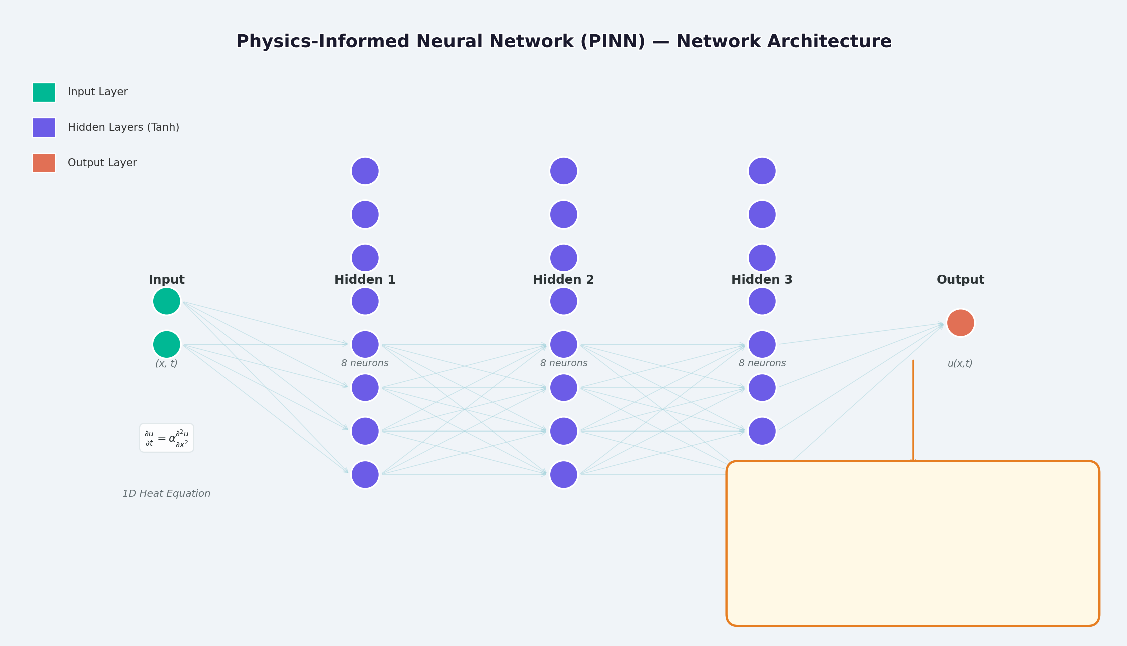
As shown in the figure above, the structure of PINN is:
Input layer : Space-time coordinates (x, t)Hidden layer : Fully connected layer + activation function (Tanh / Sigmoid)Output layer : solution of PDE u(x,t)
The key difference lies in the design of the loss function - in addition to the data fitting loss, a physical constraint loss is also added.
3. Mathematical Principles
3.1 Problem setting
Take the One-dimensional heat conduction equation as an example:
u(-1, t) = u(1, t) = 0
u(x, 0) = \sin(\pi x)
You can't use 'macro parameter character #' in math mode ### 3.2 Loss function PINN’s total loss consists of three parts: \mathcal{L}{total} = \underbrace{\mathcal{L} {PDE}}{\text{Equation residuals}} + \underbrace{\mathcal{L} {IC}}{\text{Initial conditions}} + \underbrace{\mathcal{L} {BC}}_{\text{Boundary conditions}}
f(x,t) = \frac{\partial u}{\partial t} - \alpha \frac{\partial^2 u}{\partial x^2} \quad \Rightarrow \quad \mathcal{L}{PDE} = \frac{1}{N}\sum {i=1}^{N} |f(x_i, t_i)|^2
You can't use 'macro parameter character #' in math mode > `f(x,t)` here is called <strong>residual network (physics network)</strong>, which is completely constructed by automatic differentiation and does not require any finite difference approximation. --- ## 4. PyTorch implementation ### 4.1 Environment preparation ```bash conda activate carlaTest # carlaTest 已包含: PyTorch 2.4.1 + CUDA + Matplotlib ``` ### 4.2 Complete code ```python import torch import numpy as np import matplotlib.pyplot as plt from matplotlib.animation import FuncAnimation from IPython.display import HTML, Image device = torch.device("cuda" if torch.cuda.is_available() else "cpu") print(f"Running on: {device}") # ============================================================ # 1. 定义 PINN 模型 # ============================================================ class PINN(torch.nn.Module): """Physics-Informed Neural Network""" def __init__(self, layers=[2, 32, 32, 32, 1]): super().__init__() # Xavier 初始化 self.fc = torch.nn.ModuleList([ torch.nn.Linear(layers[i], layers[i+1]) for i in range(len(layers)-1) ]) self.apply(self._init_weights) def _init_weights(self, m): if isinstance(m, torch.nn.Linear): torch.nn.init.xavier_normal_(m.weight) torch.nn.init.zeros_(m.bias) def forward(self, x): for i, fc in enumerate(self.fc[:-1]): x = torch.tanh(fc(x)) # Tanh 激活 return self.fc[-1](x) # 线性输出 # ============================================================ # 2. 精确解(用于对比) # ============================================================ alpha = 0.01 # 热扩散系数 def exact_solution(x, t): """热传导方程解析解: u(x,t) = exp(-π²αt)·sin(πx)""" return np.exp(-np.pi**2 * alpha * t) * np.sin(np.pi * x) # ============================================================ # 3. 训练函数 # ============================================================ def train_pinn(n_iterations=2000, lr=1e-3): model = PINN().to(device) optimizer = torch.optim.Adam(model.parameters(), lr=lr) history = {"total": [], "pde": [], "ic": [], "bc": []} for it in range(n_iterations): # --- PDE 残差点(内部采样)--- x_pde = (torch.rand(256, 1, device=device) * 2 - 1).requires_grad_(True) t_pde = (torch.rand(256, 1, device=device)).requires_grad_(True) # --- 初始条件点(t=0)--- x_ic = (torch.rand(64, 1, device=device) * 2 - 1) t_ic = torch.zeros(64, 1, device=device) # --- 边界条件点(x=±1)--- sign = torch.randint(0, 2, (64, 1), device=device).float() * 2 - 1 x_bc = sign # x = +1 或 x = -1 t_bc = torch.rand(64, 1, device=device) # --- 计算 PDE 残差 --- xt_pde = torch.cat([x_pde, t_pde], dim=1) u = model(xt_pde) # 自动微分:计算 u_t 和 u_xx u_t = torch.autograd.grad(u, t_pde, grad_outputs=torch.ones_like(u), create_graph=True)[0] u_x = torch.autograd.grad(u, x_pde, grad_outputs=torch.ones_like(u), create_graph=True)[0] u_xx = torch.autograd.grad(u_x, x_pde, grad_outputs=torch.ones_like(u_x), create_graph=True)[0] f = u_t - alpha * u_xx # = 0 (当网络收敛到正确解时) # --- 计算各部分损失 --- loss_pde = torch.mean(f**2) # 初始条件损失 u_ic = model(torch.cat([x_ic, t_ic], dim=1)) u_ic_exact = torch.sin(np.pi * x_ic) loss_ic = torch.mean((u_ic - u_ic_exact)**2) # 边界条件损失 u_bc = model(torch.cat([x_bc, t_bc], dim=1)) loss_bc = torch.mean(u_bc**2) # 总损失 loss = loss_pde + loss_ic + loss_bc # 反向传播 optimizer.zero_grad() loss.backward() optimizer.step() # 记录历史 if it % 50 == 0: history["total"].append(loss.item()) history["pde"].append(loss_pde.item()) history["ic"].append(loss_ic.item()) history["bc"].append(loss_bc.item()) return model, history # ============================================================ # 4. 训练 # ============================================================ print("开始训练 PINN...") model, history = train_pinn(n_iterations=2000) print(f"最终损失: {history['total'][-1]:.6f}") ``` ### 4.3 Visualization: training process ```python # === 训练损失分解动画 === fig, axes = plt.subplots(1, 2, figsize=(14, 5)) def animate(frame): step = max(1, len(history["total"]) // 50) idx = min(frame * step, len(history["total"])-1) axes[0].cla() axes[1].cla() iters = np.arange(len(history["total"])) * 50 pde_ls = history["pde"] ic_ls = history["ic"] bc_ls = history["bc"] # 左图:堆叠面积图 axes[0].fill_between(iters[:idx+1], pde_ls[:idx+1], alpha=0.4, color="#FF6B6B", label="PDE 损失") axes[0].fill_between(iters[:idx+1], np.array(pde_ls[:idx+1])+np.array(ic_ls[:idx+1]), alpha=0.4, color="#4ECDC4", label="初始条件损失") axes[0].fill_between(iters[:idx+1], np.array(pde_ls[:idx+1])+np.array(ic_ls[:idx+1])+np.array(bc_ls[:idx+1]), alpha=0.4, color="#45B7D1", label="边界条件损失") axes[0].set_yscale("log") axes[0].set_xlabel("迭代次数") axes[0].set_ylabel("损失值 (对数坐标)") axes[0].legend(loc="upper right") axes[0].grid(True, alpha=0.3) axes[0].set_title("损失分量演化(堆叠面积图)") # 右图:分线对比 axes[1].semilogy(iters[:idx+1], pde_ls[:idx+1], "r-", lw=2, label="PDE") axes[1].semilogy(iters[:idx+1], ic_ls[:idx+1], "g--", lw=2, label="初始条件") axes[1].semilogy(iters[:idx+1], bc_ls[:idx+1], "b:", lw=2, label="边界条件") axes[1].scatter([iters[idx]], [history["total"][idx]], color="purple", s=100, zorder=5) axes[1].set_xlabel("迭代次数") axes[1].set_ylabel("损失值 (对数坐标)") axes[1].legend(loc="upper right") axes[1].grid(True, alpha=0.3) axes[1].set_title("各损失分量对比") ani = FuncAnimation(fig, animate, frames=50, interval=150) ani.save("pinn_loss_components.gif", writer="pillow", fps=6, dpi=100) ``` --- ## 5. Visualize results ### 5.1 Convergence process of solution 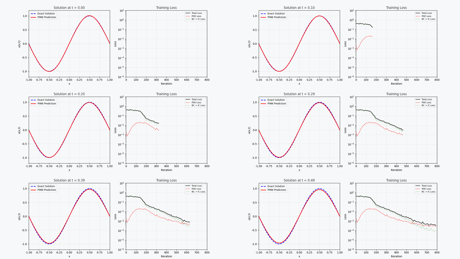 The figure above shows the process of PINN gradually approaching the exact solution during the training process: - <strong>Left picture</strong>: Solution curve at time t=0.5, the red dotted line is PINN prediction, and the blue solid line is the exact solution - <strong>Middle picture</strong>: Training loss (log scale), you can see that the three losses decrease collaboratively - <strong>Right image</strong>: Complete (x,t) solution field predicted by PINN ### 5.2 Loss function decomposition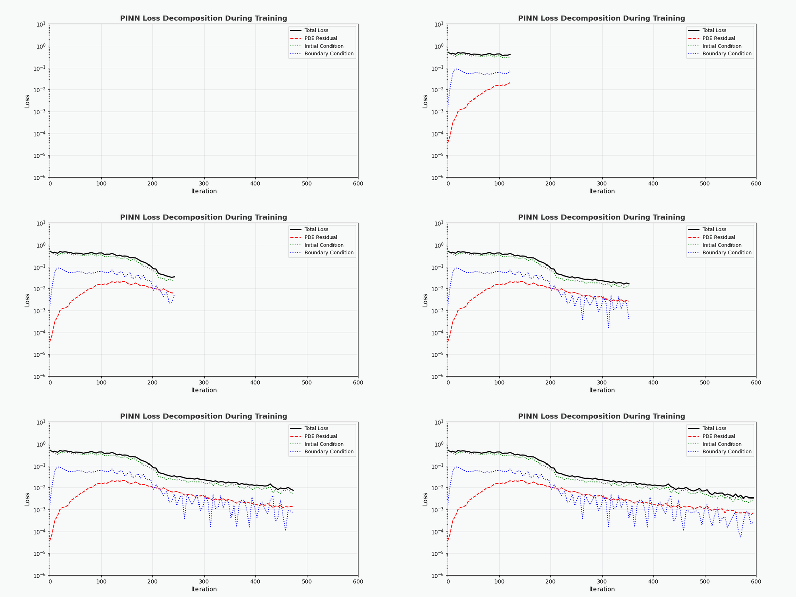 As can be seen from the loss decomposition animation: - <strong>PDE loss (red)</strong> dropped the fastest, indicating that the network quickly learned the laws of physics - <strong>Boundary condition loss (blue)</strong> is usually the smallest because the boundary condition constraints are the simplest - The three losses eventually stabilize, indicating that the network has converged --- ## 6. Advantages of PINN | Properties | Traditional Numerical Methods (FEM/FDM) | PINN | |------|------------------------|------| | Grid generation | Requires fine grid, high dimensionality is difficult | <strong>No grid required</strong>, Random sampling | | Derivative accuracy | Relies on differential approximation, with truncation errors | <strong>Automatic differentiation</strong>, arbitrary precision | | Irregular areas | Complex meshing | <strong>Natural support</strong> for arbitrary geometries | | Inverse problem | Re-solver required | <strong>End-to-end</strong> gradient optimization | | High-dimensional problems | Curse of dimensionality | <strong>Scalable</strong> | --- ## 7. Limitations and challenges of PINN > PINN is not a panacea - it has its own unique limitations. ### 7.1 Training Difficulties - <strong>Mode Collapse</strong>: When the PDE has multiple solutions, PINN may only learn one of them - <strong>Vanishing gradient</strong>: The gradient of high-order derivatives (such as u_xxxx) may be extremely small in deep networks - <strong>Hyperparameter sensitivity</strong>: Network depth, learning rate, and sampling strategy have a significant impact on the results. ### 7.2 Solution accuracy - Neural networks have poor accuracy in <strong>high frequency solutions</strong> (such as oscillation solutions) - Boundary layers and singularities require special processing (adaptive sampling, period expansion, etc.) ### 7.3 Computational efficiency - PINN tends to be<strong>slower</strong> on simple PDEs than mature numerical libraries (e.g. FEniCS, COMSOL) - GPU utilization is not as high as dedicated numerical code ### 7.4 Directions for improvement- <strong>Adaptive Sampling</strong>: Multi-sampling in areas with large errors (such as Residual-based Adaptive Refinement) - <strong>DeepONet</strong>: Operator Network, directly learn PDE solution operators - <strong>Fourier Neural Operator (FNO)</strong>: Frequency domain neural operator, better for high-dimensional problems - <strong>HP-VPINN</strong>: PINN based on variational form, higher accuracy --- ## 8. Complete training code (ready to run) ```python """ PINN 求解一维热传导方程 conda activate carlaTest python pinn_heat_equation.py """ import torch, numpy as np, matplotlib.pyplot as plt device = torch.device("cuda" if torch.cuda.is_available() else "cpu") alpha = 0.01 class PINN(torch.nn.Module): def __init__(self): super().__init__() self.net = torch.nn.Sequential( torch.nn.Linear(2, 32), torch.nn.Tanh(), torch.nn.Linear(32, 32), torch.nn.Tanh(), torch.nn.Linear(32, 32), torch.nn.Tanh(), torch.nn.Linear(32, 1) ) def forward(self, x): return self.net(x) model = PINN().to(device) opt = torch.optim.Adam(model.parameters(), lr=1e-3) for it in range(2000): x_pde = (torch.rand(256,1,device=device)*2-1).requires_grad_(True) t_pde = (torch.rand(256,1,device=device)).requires_grad_(True) x_ic = (torch.rand(64,1,device=device)*2-1) t_ic = torch.zeros(64,1,device=device) x_bc = (torch.randint(0,2,(64,1),device=device).float()*2-1) t_bc = torch.rand(64,1,device=device) xt = torch.cat([x_pde,t_pde],dim=1) u = model(xt) u_t = torch.autograd.grad(u,t_pde,torch.ones_like(u),create_graph=True)[0] u_x = torch.autograd.grad(u,x_pde,torch.ones_like(u),create_graph=True)[0] u_xx = torch.autograd.grad(u_x,x_pde,torch.ones_like(u_x),create_graph=True)[0] loss = (torch.mean((u_t-alpha*u_xx)**2) + torch.mean((model(torch.cat([x_ic,t_ic],1))-torch.sin(np.pi*x_ic))**2) + torch.mean(model(torch.cat([x_bc,t_bc],1))**2)) opt.zero_grad(); loss.backward(); opt.step() if it%200==0: print(f"Iter {it:5d} | Loss: {loss.item():.6f}") # 测试 x_test = torch.linspace(-1,1,100,device=device).reshape(-1,1) t_test = torch.ones(100,1,device=device)*0.5 u_pred = model(torch.cat([x_test,t_test],1)).cpu().detach().numpy() u_true = np.exp(-np.pi**2*alpha*0.5)*np.sin(np.pi*x_test.cpu().numpy()) plt.figure(figsize=(8,4)) plt.plot(x_test.cpu(),u_true,"b-",lw=2,label="精确解") plt.plot(x_test.cpu(),u_pred,"r--",lw=2,label="PINN 预测") plt.legend(); plt.title("t=0.5 时刻的热传导方程解") plt.savefig("pinn_result.png",dpi=150) print("结果已保存!") ``` --- ## 9. Summary PINN embeds <strong>physical prior</strong> into the training process of neural networks, opening up a new paradigm of "physics-driven deep learning". Its core innovation is not the network structure, but the design of the loss function - precisely imposing physical constraints with automatic differentiation. Despite challenges such as difficulty in training and limited accuracy, PINN has demonstrated unique value in the following scenarios: - <strong>High-dimensional PDE</strong> (traditional method dimensionality disaster) - <strong>Inverse problem</strong> (parameter identification, data assimilation) - <strong>Uncertainty quantification</strong> (combined with Bayesian methods) > If you want to explore further, it is recommended to start with the [DeepXDE](https://deepxde.readthedocs.io/) library, which encapsulates a large number of PINN variants and adaptive sampling strategies. ---<strong>Reference papers:</strong> 1. Raissi, M., Perdikaris, P., & Karniadakis, G. E. (2019). *Physics-informed neural networks: A deep learning framework for solving forward and inverse problems involving nonlinear partial differential equations.* Journal of Computational Physics, 378, 686-707. 2. Lu, L., et al. (2021). *DeepONet: Learning nonlinear operators for identifying differential equations based on the universal approximation theorem of operators.* Nature Machine Intelligence, 3(3), 218-229. 3. Li, Z., Kovachki, N., Azizzadenesheli, K., Liu, B., Bhattacharya, K., Stuart, A., & Anandkumar, A. (2020). *Fourier neural operator for parametric partial differential equations.* arXiv preprint arXiv:2010.08895.